一、什么是自動編碼器？

自編碼器是開發(fā)無監(jiān)督學習模型的主要方式之一。但什么是自動編碼器？

成都創(chuàng)新互聯(lián)公司專注于企業(yè)營銷型網站建設、網站重做改版、滿城網站定制設計、自適應品牌網站建設、成都h5網站建設、商城網站定制開發(fā)、集團公司官網建設、外貿網站建設、高端網站制作、響應式網頁設計等建站業(yè)務，價格優(yōu)惠性價比高，為滿城等各大城市提供網站開發(fā)制作服務。

簡而言之，自動編碼器通過接收數(shù)據、壓縮和編碼數(shù)據，然后從編碼表示中重構數(shù)據來進行操作。對模型進行訓練，直到損失最小化并且盡可能接近地再現(xiàn)數(shù)據。通過這個過程，自動編碼器可以學習數(shù)據的重要特征。

自動編碼器是由多個層組成的神經網絡。自動編碼器的定義方面是輸入層包含與輸出層一樣多的信息。輸入層和輸出層具有完全相同數(shù)量的單元的原因是自動編碼器旨在復制輸入數(shù)據。然后分析數(shù)據并以無監(jiān)督方式重建數(shù)據后輸出數(shù)據副本。

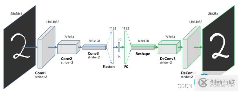
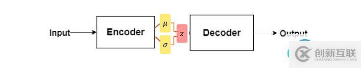
通過自動編碼器的數(shù)據不僅僅是從輸入直接映射到輸出。自動編碼器包含三個組件：壓縮數(shù)據的編碼（輸入）部分、處理壓縮數(shù)據（或瓶頸）的組件和解碼器（輸出）部分。當數(shù)據被輸入自動編碼器時，它會被編碼，然后壓縮到更小的尺寸。然后對網絡進行編碼/壓縮數(shù)據的訓練，并輸出該數(shù)據的重建。

? 神經網絡學習了輸入數(shù)據的“本質”或最重要的特征，這是自動編碼器的核心價值。訓練完網絡后，訓練好的模型就可以合成相似的數(shù)據，并添加或減去某些目標特征。例如，您可以在加了噪聲的圖像上訓練自動編碼器，然后使用經過訓練的模型從圖像中去除噪聲。

自編碼器的應用包括：異常檢測、數(shù)據去噪（例如圖像、音頻）、圖像著色、圖像修復、信息檢索等、降維等。

二、自動編碼器的架構

自動編碼器基本上可以分為三個不同的組件：編碼器、瓶頸和解碼器。

編碼器：編碼器是一個前饋、全連接的神經網絡，它將輸入壓縮為潛在空間表示，并將輸入圖像編碼為降維的壓縮表示。壓縮后的圖像是原始圖像的變形版本。

code：網絡的這一部分包含輸入解碼器的簡化表示。

解碼器：解碼器和編碼器一樣也是一個前饋網絡，結構與編碼器相似。該網絡負責將輸入從代碼中重建回原始維度。

首先，輸入通過編碼器進行壓縮并存儲在稱為code的層中，然后解碼器從代碼中解壓縮原始輸入。自編碼器的主要目標是獲得與輸入相同的輸出。

通常情況下解碼器架構是編碼器的鏡像，但也不是絕對的。唯一的要求是輸入和輸出的維度必須相同。

三、自動編碼器的類型 1、卷積自動編碼器

卷積自動編碼器是通用的特征提取器。卷積自編碼器是采用卷積層代替全連接層，原理和自編碼器一樣，對輸入的象征進行降采樣以提供較小維度潛在表示，并強制自編碼器學習象征的壓縮版本。

2、去噪自動編碼器

這種類型的自動編碼器適用于部分損壞的輸入，并訓練以恢復原始未失真的圖像。如上所述，這種方法是限制網絡簡單復制輸入的有效方法。

目標是網絡將能夠復制圖像的原始版本。通過將損壞的數(shù)據與原始數(shù)據進行比較，網絡可以了解數(shù)據的哪些特征最重要，哪些特征不重要/損壞。換句話說，為了讓模型對損壞的圖像進行去噪，它必須提取圖像數(shù)據的重要特征。

3、收縮自動編碼器

收縮自動編碼器的目標是降低表示對訓練輸入數(shù)據的敏感性。 為了實現(xiàn)這一點，在自動編碼器試圖最小化的損失函數(shù)中添加一個正則化項或懲罰項。

收縮自動編碼器通常僅作為其他幾種自動編碼器節(jié)點存在。去噪自動編碼器使重建函數(shù)抵抗輸入的小但有限大小的擾動，而收縮自動編碼器使特征提取函數(shù)抵抗輸入的無窮小擾動。

4、變分自動編碼器

Variational Autoencoders，這種類型的自動編碼器對潛在變量的分布做出了假設，并在訓練過程中使用了隨機梯度變分貝葉斯估計器。

訓練時，編碼器為輸入圖像的不同特征創(chuàng)建潛在分布。

本質上，該模型學習了訓練圖像的共同特征，并為它們分配了它們發(fā)生的概率。然后可以使用概率分布對圖像進行逆向工程，生成與原始訓練圖像相似的新圖像。?

這種類型的自動編碼器可以像GAN一樣生成新圖像。由于 VAE 在生成行為方面比GAN更加靈活和可定制，因此它們適用于任何類型的藝術生成。

四、自動編碼器與PCA有何不同？

PCA 和自動編碼器是降低特征空間維數(shù)的兩種流行方法。

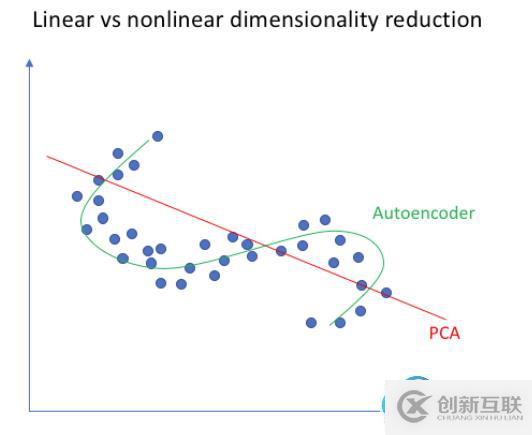
PCA 從根本上說是一種線性變換，但自動編碼器可以描述復雜的非線性過程。如果我們要構建一個線性網絡（即在每一層不使用非線性激活函數(shù)），我們將觀察到與 PCA 中相似的降維。

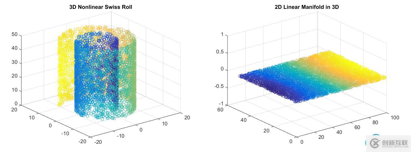
PCA 試圖發(fā)現(xiàn)描述原始數(shù)據的低維超平面，而自動編碼器能夠學習非線性流形（流形簡單地定義為連續(xù)的、不相交的表面）。

與自動編碼器相比，PCA 的計算速度更快且成本更低。但由于參數(shù)數(shù)量多，自編碼器容易過擬合。

五、自編碼器與GAN有何不同？

? 1、兩者都是生成模型。AE試圖找到以特定輸入（更高維度）為條件的數(shù)據的低維表示，而GAN 試圖創(chuàng)建足以概括以鑒別器為條件的真實數(shù)據分布的表示。

? 2、雖然它們都屬于無監(jiān)督學習的范疇，但它們是解決問題的不同方法。

GAN 是一種生成模型——它應該學習生成數(shù)據集的新樣本。

變分自動編碼器是生成模型，但普通的自動編碼器只是重建它們的輸入，不能生成真實的新樣本。

https://www.quora.com/What-is-the-difference-between-Generative-Adversarial-Networks-and-Autoencodershttps://www.quora.com/What-is-the-difference-between-Generative-Adversarial-Networks-and-Autoencoders

六、實例1：去噪自動編碼器 1、概述

? 去噪自動編碼器的一個應用的例子是預處理圖像以提高光學字符識別 (OCR) 算法的準確性。如果您以前應用過OCR，就會知道一丁點錯誤的噪聲（例如，打印機墨水污跡、掃描過程中的圖像質量差等）都會嚴重影響OCR識別的效果。使用去噪自編碼器，可以自動對圖像進行預處理，提高質量，從而提高OCR識別算法的準確性。

? 我們這里故意向MNIST訓練圖像添加噪聲。目的是使我們的自動編碼器能夠有效地從輸入圖像中去除噪聲。

2、參考代碼

? 創(chuàng)建autoencoder_for_denoising.py文件，插入以下代碼。

# import the necessary packages
from tensorflow.keras.layers import BatchNormalization
from tensorflow.keras.layers import Conv2D
from tensorflow.keras.layers import Conv2DTranspose
from tensorflow.keras.layers import LeakyReLU
from tensorflow.keras.layers import Activation
from tensorflow.keras.layers import Flatten
from tensorflow.keras.layers import Dense
from tensorflow.keras.layers import Reshape
from tensorflow.keras.layers import Input
from tensorflow.keras.models import Model
from tensorflow.keras import backend as K
import numpy as np

class ConvAutoencoder:
	@staticmethod
	def build(width, height, depth, filters=(32, 64), latentDim=16):
		# initialize the input shape to be "channels last" along with
		# the channels dimension itself
		# channels dimension itself
		inputShape = (height, width, depth)
		chanDim = -1
		# define the input to the encoder
		inputs = Input(shape=inputShape)
		x = inputs

		# loop over the number of filters
		for f in filters:
			# apply a CONV =>RELU =>BN operation
			x = Conv2D(f, (3, 3), strides=2, padding="same")(x)
			x = LeakyReLU(alpha=0.2)(x)
			x = BatchNormalization(axis=chanDim)(x)
		# flatten the network and then construct our latent vector
		volumeSize = K.int_shape(x)
		x = Flatten()(x)
		latent = Dense(latentDim)(x)
		# build the encoder model
		encoder = Model(inputs, latent, name="encoder")

		# start building the decoder model which will accept the
		# output of the encoder as its inputs
		latentInputs = Input(shape=(latentDim,))
		x = Dense(np.prod(volumeSize[1:]))(latentInputs)
		x = Reshape((volumeSize[1], volumeSize[2], volumeSize[3]))(x)
		# loop over our number of filters again, but this time in
		# reverse order
		for f in filters[::-1]:
			# apply a CONV_TRANSPOSE =>RELU =>BN operation
			x = Conv2DTranspose(f, (3, 3), strides=2, padding="same")(x)
			x = LeakyReLU(alpha=0.2)(x)
			x = BatchNormalization(axis=chanDim)(x)
		# apply a single CONV_TRANSPOSE layer used to recover the
		# original depth of the image
		x = Conv2DTranspose(depth, (3, 3), padding="same")(x)
		outputs = Activation("sigmoid")(x)
		# build the decoder model
		decoder = Model(latentInputs, outputs, name="decoder")
		# our autoencoder is the encoder + decoder
		autoencoder = Model(inputs, decoder(encoder(inputs)), name="autoencoder")
		# return a 3-tuple of the encoder, decoder, and autoencoder
		return (encoder, decoder, autoencoder)


# set the matplotlib backend so figures can be saved in the background
import matplotlib
matplotlib.use("Agg")
# import the necessary packages
from tensorflow.keras.optimizers import Adam
from tensorflow.keras.datasets import mnist
import matplotlib.pyplot as plt
import numpy as np
import argparse
import cv2
# construct the argument parse and parse the arguments
ap = argparse.ArgumentParser()
ap.add_argument("-s", "--samples", type=int, default=8, help="# number of samples to visualize when decoding")
ap.add_argument("-o", "--output", type=str, default="output.png", help="path to output visualization file")
ap.add_argument("-p", "--plot", type=str, default="plot.png", help="path to output plot file")
args = vars(ap.parse_args())

# initialize the number of epochs to train for and batch size
EPOCHS = 25
BS = 32
# load the MNIST dataset
print("[INFO] loading MNIST dataset...")
((trainX, _), (testX, _)) = mnist.load_data()
# add a channel dimension to every image in the dataset, then scale
# the pixel intensities to the range [0, 1]
trainX = np.expand_dims(trainX, axis=-1)
testX = np.expand_dims(testX, axis=-1)
trainX = trainX.astype("float32") / 255.0
testX = testX.astype("float32") / 255.0

# sample noise from a random normal distribution centered at 0.5 (since
# our images lie in the range [0, 1]) and a standard deviation of 0.5
trainNoise = np.random.normal(loc=0.5, scale=0.5, size=trainX.shape)
testNoise = np.random.normal(loc=0.5, scale=0.5, size=testX.shape)
trainXNoisy = np.clip(trainX + trainNoise, 0, 1)
testXNoisy = np.clip(testX + testNoise, 0, 1)

# construct our convolutional autoencoder
print("[INFO] building autoencoder...")
(encoder, decoder, autoencoder) = ConvAutoencoder.build(28, 28, 1)
opt = Adam(lr=1e-3)
autoencoder.compile(loss="mse", optimizer=opt)
# train the convolutional autoencoder
H = autoencoder.fit(trainXNoisy, trainX, validation_data=(testXNoisy, testX), epochs=EPOCHS, batch_size=BS)
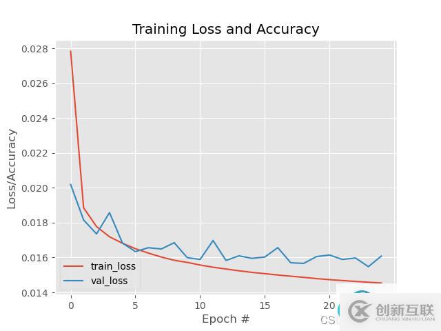
# construct a plot that plots and saves the training history
N = np.arange(0, EPOCHS)
plt.style.use("ggplot")
plt.figure()
plt.plot(N, H.history["loss"], label="train_loss")
plt.plot(N, H.history["val_loss"], label="val_loss")
plt.title("Training Loss and Accuracy")
plt.xlabel("Epoch #")
plt.ylabel("Loss/Accuracy")
plt.legend(loc="lower left")
plt.savefig(args["plot"])


# use the convolutional autoencoder to make predictions on the
# testing images, then initialize our list of output images
print("[INFO] making predictions...")
decoded = autoencoder.predict(testXNoisy)
outputs = None
# loop over our number of output samples
for i in range(0, args["samples"]):
	# grab the original image and reconstructed image
	original = (testXNoisy[i] * 255).astype("uint8")
	recon = (decoded[i] * 255).astype("uint8")
	# stack the original and reconstructed image side-by-side
	output = np.hstack([original, recon])
	# if the outputs array is empty, initialize it as the current
	# side-by-side image display
	if outputs is None:
		outputs = output
	# otherwise, vertically stack the outputs
	else:
		outputs = np.vstack([outputs, output])
# save the outputs image to disk
cv2.imwrite(args["output"], outputs)

? 然后輸入以下命令進行訓練。

python train_denoising_autoencoder.py --output output_denoising.png --plot plot_denoising.png

3、訓練結果

? 經過25epoch的訓練結果。

對應的去噪結果圖，左邊是添加噪聲的原始MNIST數(shù)字，而右邊是去噪自動編碼器的輸出——可以看到去噪自動編碼器能夠在消除噪音的同時從圖像中恢復原始信號。

你是否還在尋找穩(wěn)定的海外服務器提供商？創(chuàng)新互聯(lián)www.cdcxhl.cn海外機房具備T級流量清洗系統(tǒng)配攻擊溯源，準確流量調度確保服務器高可用性，企業(yè)級服務器適合批量采購，新人活動首月15元起，快前往官網查看詳情吧

本文名稱：機器學習筆記-自動編碼器autoencoder-創(chuàng)新互聯(lián)
標題來源：http://www.chinadenli.net/article40/dosgho.html

成都網站建設公司_創(chuàng)新互聯(lián)，為您提供品牌網站制作、云服務器、手機網站建設、網站導航、外貿建站、網站排名

廣告

聲明：本網站發(fā)布的內容（圖片、視頻和文字）以用戶投稿、用戶轉載內容為主，如果涉及侵權請盡快告知，我們將會在第一時間刪除。文章觀點不代表本網站立場，如需處理請聯(lián)系客服。電話：028-86922220；郵箱：631063699@qq.com。內容未經允許不得轉載，或轉載時需注明來源： 創(chuàng)新互聯(lián)